Use Conditional Formatting in Cube Views to visually explore and analyze data. You can highlight cells or ranges of cells, identify key values, and represent data using data bars, color scales, and icon sets that correspond to specific variations in the data. If there are any existing formats prior to applying Conditional Formatting, they will be retained if the range of cells containing the conditional formats do not meet the conditions of the rule. All styles from the cube view and the selection styles that had been previously applied to that range are overridden by conditional formatting.
Create Conditional Formatting in an Existing or New Cube View
-
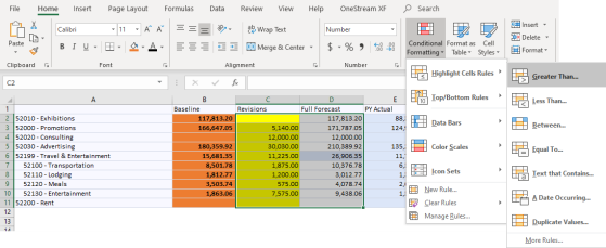
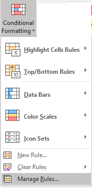
Click Home > Conditional Formatting > Highlight Cells Rules > Greater Than.
-
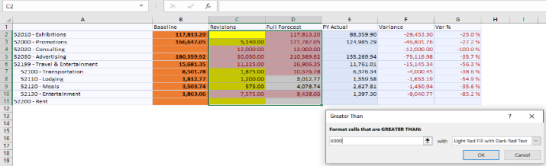
Enter 6000 and click OK.
-
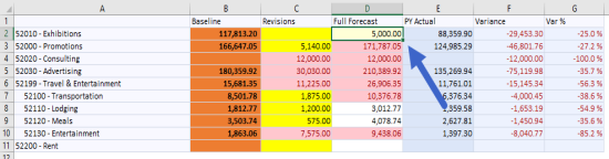
Go to OneStream and click Refresh Sheet to see that your changes have been applied.
-
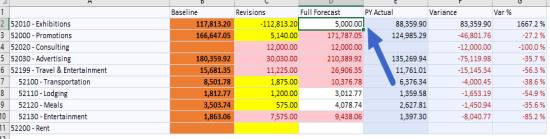
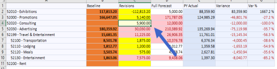
If you make a change that is different than the value in the database, the cell will change to pale yellow, until you refresh or submit.
-
If you submit, it will revert to the formatting that was in the cube view since it is no longer greater than 6000.
-
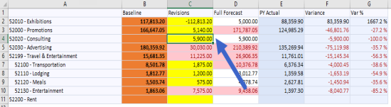
If you make a change to a cell that has conditional formatting and a selection style,
when you submit, it will convert back to the selection style since it is no longer greater than 6000.
-
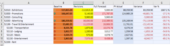
To add icons, go Home > Conditional Formatting > Icon Sets and select the icons to use, in this example, select the arrows.
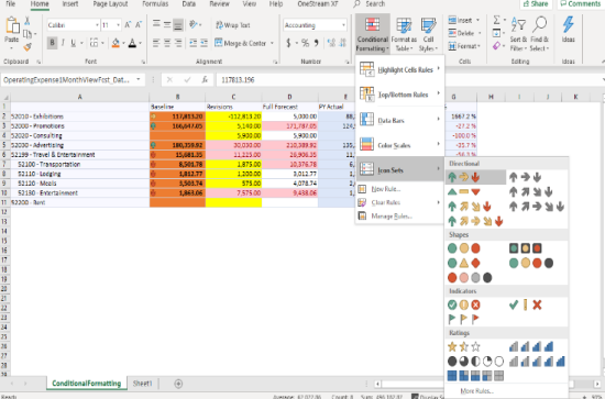
-
The icons are part of the cube view.
-
You can also create, edit, delete, and view all conditional formatting rules.
-
If you save the workbook, the conditional formatting is saved.


